Article Text

Abstract
Myopia is a global healthcare concern and effective analyses of dioptric power are important in evaluating potential treatments involving surgery, orthokeratology, drugs such as low-dose (0.05%) atropine and gene therapy. This paper considers issues of concern when analysing refractive state such as data normality, transformations, outliers and anisometropia. A brief review of methods for analysing and representing dioptric power is included but the emphasis is on the optimal approach to understanding refractive state (and its variation) in addressing pertinent clinical and research questions.
Although there have been significant improvements in the analysis of refractive state, areas for critical consideration remain and the use of power matrices as opposed to power vectors is one such area. Another is effective identification of outliers in refractive data. The type of multivariate distribution present with samples of dioptric power is often not considered. Similarly, transformations of samples (of dioptric power) towards normality and the effects of such transformations are not thoroughly explored. These areas (outliers, normality and transformations) need further investigation for greater efficacy and proper inferences regarding refractive error. Although power vectors are better known, power matrices are accentuated herein due to potential advantages for statistical analyses of dioptric power such as greater simplicity, completeness, and improved facility for quantitative and graphical representation of refractive state.
- optics and refraction
- vision
- public health
Data availability statement
Data are available on reasonable request.
This is an open access article distributed in accordance with the Creative Commons Attribution Non Commercial (CC BY-NC 4.0) license, which permits others to distribute, remix, adapt, build upon this work non-commercially, and license their derivative works on different terms, provided the original work is properly cited, appropriate credit is given, any changes made indicated, and the use is non-commercial. See: http://creativecommons.org/licenses/by-nc/4.0/.
Statistics from Altmetric.com
Introduction
Instantaneous dioptric power (a 2×2 matrix, F) where variation over time is momentarily ignored is fundamentally a four-variate quantity1 and any suitable analysis must take into consideration that power is quantifiable using four unique quantities or numbers. (eg, the instantaneous power of the human eye, a thick optical system, is four- dimensional).
Refractive behaviour or the variation over time of instantaneous refractive state (a three-dimensional quantity defined as the dioptric power of a thin lens with three df, ie, sphere, cylinder and its axis)2 is a multivariate concern. Factors such as age or visual acuity add dimensions in any analytical situation involving refractive behaviour. The logical mathematical approach for such multivariate quantities is via matrices (asymmetric or sometimes symmetric) and the various operations of linear algebra.1 2 Sometimes symmetric matrices2 are applicable and in most clinical situations such as with refractive state this simplification applies. This review will apply experimental data to highlight a few critical issues for further investigation and theoretical development in the years to come concerning dioptric power and its analysis in scientific studies.
Early attempts to understand dioptric power involved the use of optometric vectors (by Gartner3) where the angles of the cylinder axes were doubled for a more mathematically appropriate Cartesian two-dimensional space with limits of 0°–360°. Gartner limited his analysis to cylinder only but Fick published three papers4–6 in 1972–1973 that introduced the ideas of applying matrices and linear algebra to dioptric power while Long7 and Keating,8 9 working independently, provided conversion equations from clinical notation (F s F c A) to power matrices and also for the necessary inverse operations.
Harris10 mentions the need for a system of analysis allowing for invariance of power under sphero-cylindrical transposition and also describes methods for calculating squares of a power10 and performing mathematical operations necessary for effective determination of quantities such as means and variances when analysing and comparing samples of dioptric power.10–16 Harris et al describe methods for ellipsoids or surfaces of constant probability density (SCPD) when comparing distributions17 18 and for testing samples of dioptric power for variance14 and departure from normality that involve profiles of skewness, kurtosis and standardised mean deviation (see Harris and Malan19 for further developments in that area and also trajectories for dioptric power.20 This foundation for understanding distributions of power and transformations towards normality is further developed by Harris and Blackie21 22 where concepts such as Mardia’s multivariate skewness and kurtosis23 are employed including normality plots (marginal and χ2) for refractive state.21 22 Hypothesis tests, integral to understanding experimental effects in the context of dioptric power, are described by Harris.12 13 15
Thibos et al referred to power vectors24 with three terms, namely M, J 0 and J 45 and an advantage of these vectors compared with those of Gartner is that they cope with the three-dimensional (3D) nature of symmetric power but not for four-dimensional asymmetric power.1 2 25 (Others such as Naeser and Hjortdal26 use KP(90) and KP(135) that are the same as J 0 and J 45.) See Harris for a comparison of power vectors and power matrices.27 Refractive behaviour28 in Euclidean three-space can be studied using such mathematical and graphical methods with trajectories,20 comets (to link paired measurements),28 and other methods such as SCPD17 18 including also meridional profiles of various types.14 19 21 28 29 Polar plots for variance of dioptric power were first described by Harris and van Gool30 31 and van Gool used them (and much of the aforementioned methodology) for an analysis that involved ocular accommodation and leads or lags of accommodation to near stimuli.31 (Some of these methods will be illustrated later.)
Other methods to analyse and understand refractive behaviour include that of Alpins32 33 where vectors are similarly applied to, for example, investigate changes in specifically astigmatism after corneal surgery.34–36 Vector magnitudes and directions are represented using polar plots and surgical outcomes can be expressed in terms of difference vectors, and target induced and surgically induced astigmatism vectors.
Researchers have applied the concepts of a more effective analytical and scientific approach to studies of refractive behaviour and examples include Raasch,37 Kaye et al 38 39 and others concerned with reproducibility of measures of refractive state40 and issues relating to intraocular lens (IOL) implants.41–44 See also MacKenzie and Harris45 and MacKenzie46 for the application of multivariate methods and power matrices to intraocular implants and their uses in ameliorating refractive errors and cataract. Harris1 16 47 48 and MacKenzie,45 46 van Gool,49 Evans50 51 and others52 53 applied these theoretical ideas for linear optical systems (and ray behaviour through such systems). Since this area is the subject for another review they are not further described here.
Possible relationships between refractive behaviour and visual acuity are explored by Harris and Rubin but this multidimensional topic is not further considered here.54 55 Power vectors and power matrices and the analytical methods as explained and described mathematically below have been applied to a diverse range of clinical and experimental topics20–74 including autorefraction in adults,28–31 56 57 children,58 66 keratometric variation,59–61 comparisons of methods to measure refractive behaviour in relation to age62 63 and other factors including also luminance of targets within autorefractors65 and wavefront aberrometry,66 interocular mirror symmetry,67 cycloplegia,64 68 keratoconus,69 70 measurement error and uncertainty,64 71 72 anisometropia73 and refractive surgery.74
Dioptric power and refractive behaviour
Refractive state has three quantities; the powers of a sphere (F s or S) and cylinder (F c or C) and its axis (A) and the combination of quantities F s F c A (or S C A) is frequently referred to as clinical or conventional notation. In this paper, we shall describe the dioptric power matrix as well as two coordinate power vectors and their relationship to the power matrix. Transformations from clinical notation to power matrices1 2 7–9 27 37–39 or power vectors1–6 24 26 27 32–39 is relatively simple. The 2×2 dioptric power matrix1 4–9 is given by:
 (1)
(1)
Throughout the paper, bold letters are used to indicate matrices (capital letters) or vectors (lowercase letters), while scalar variables are indicated with italics. For thin optical systems, the entries for the 2×2 symmetric power matrix F in equation 1 are determined via equations from Long7 (or equations from Fick4–6):
 (2)
(2)
 (3)
(3)
and
 (4)
(4)
The entry f
11 in F is effectively the power in the reference meridian (usually horizontal for quantification of cylinder axis) while f
22 is the power in the meridian perpendicular to the reference meridian (usually the vertical meridian).7 The off-diagonal entries f
12 and f
21 are the torsional powers8 in the reference meridian (usually but not always horizontal) and meridian perpendicular to that reference meridian (usually but not always vertical). For thin systems and symmetric F,  and there are effectively only three coefficients of power; two (f
11 and f
12) are referred to as the curvital coefficients and one (
and there are effectively only three coefficients of power; two (f
11 and f
12) are referred to as the curvital coefficients and one ( ) as the torsional coefficient of power. Conventionally, the reference meridian is horizontal, however, it is possible to take any other meridian as reference2 16 and this can be useful with meridional plots14 19 28–31 such as will be included later.
To perform the inverse operation (from F to clinical notation) equations 7–9 from Keating8 (or equations from Fick6 can be used after first determining the trace (t) and determinant (d) of F 2×2:
 (5)
(5)
 (6)
(6)
 (7)
(7)
 (8)
(8)
 (9)
(9)
For an astigmatic system, the eigenvalues of F are the powers (F 1 and F 2) along the principal meridians and the eigenvectors correspond to the principal directions or meridians (A 1 and A 2) for those powers.1 7 9 For a symmetric matrix, the eigenvectors are perpendicular to each other, however, for an asymmetric matrix, such as may be found with the power of thick optical systems, the eigenvalues are not perpendicular. Power obtained from the eigenstructure conforms to common meridional representations of power in ophthalmology and optometry, such as the optical or power cross used to represent powers of thin lenses or surfaces, for example, the corneal via central keratometric values.1 Any powers (F 1 and F 2) along principal meridians (A 1 and A 2) can be represented using principal meridional representation where F 1{along A 1} F 2{along A 2} is used. (Given that the meridians are always orthogonal one can exclude the last part, that is, {along A 2}.)75
Two coordinate vectors have been proposed, each with a different basis. For symmetric dioptric power, the basis will always have three components. Historically, the first, coordinate vector h, was proposed by Harris2 10–13 in 1990 to graphically represent power and the second, power vector t, by Thibos et al 24 in 1997. While vector t has gained popularity, both coordinate vectors are useful for analysing dioptric power and both represent symmetric dioptric power space (SDPS).
Coordinate vector h as a 3×1 column vector is2 10–13:
 (10)
(10)
with basis:

such that
 ,
,
is the symmetric dioptric power. The coefficients are the coordinates of F with respect to the basis γ .1
There are two interpretations for coordinate vector h, that is, the meridional and component interpretations.2 20 In the meridional interpretation, h
1 and h
3 are, respectively, curvital powers in the reference (or usually horizontal meridian) and in the meridian perpendicular to the reference meridian while h
2 is the scaled (f
21 is multiplied by the factor  ) torsional power along the reference meridian. Thus, within any meridian there are two types of power (curvital and torsional). In the component interpretation, h
1 and h
3 are respectively two component cylinder powers, also in the reference or horizontal meridian and in the meridian perpendicular to the reference meridian while h
2 is the scaled power of a Jackson cross cylinder (JCC) with principal axes at 45° and 135°. Harris refers to spherical powers as scalar or stigmatic powers16 75 and JCC or Jacksonian powers are referred to by Harris (and coworkers) as antiscalar or antistigmatic powers.76
) torsional power along the reference meridian. Thus, within any meridian there are two types of power (curvital and torsional). In the component interpretation, h
1 and h
3 are respectively two component cylinder powers, also in the reference or horizontal meridian and in the meridian perpendicular to the reference meridian while h
2 is the scaled power of a Jackson cross cylinder (JCC) with principal axes at 45° and 135°. Harris refers to spherical powers as scalar or stigmatic powers16 75 and JCC or Jacksonian powers are referred to by Harris (and coworkers) as antiscalar or antistigmatic powers.76
The terms curvital and torsional can best be described using a single refracting surface, such as the anterior cornea, where each meridian of that corneal surface has curvature (think of bending a thin strip of paper along or in the direction of the meridian) but also twist or torsion (think of twisting a thin strip of paper where each hand at the ends of the strip rotates in an opposite direction). Instead of a sphere and cylinder with its corresponding axis as in clinical notation, coordinate vector h in the component interpretation can be thought of as the powers of two orthogonal cylinder powers with axis parallel (h 3) or perpendicular (h 3) to the reference meridian and one JCC or antiscalar power (h 2), with principal meridians at 45° and 135°.
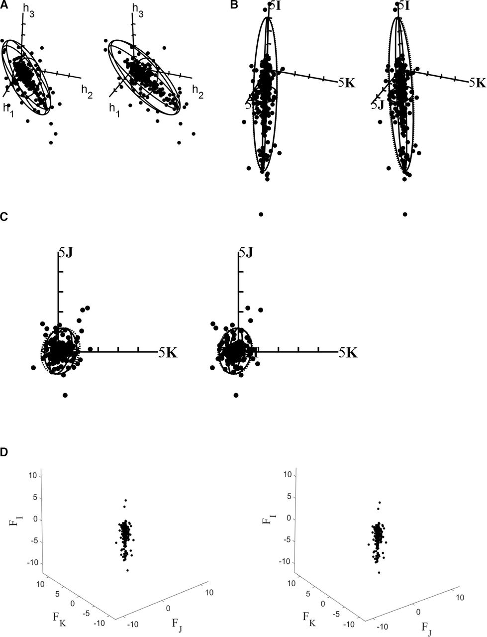
For one or more powers, it is possible then to use these coordinates (ie, h 1, h 2 and h 3 in equation 10) for plots in SDPS, a Euclidean 3-space2 where each symmetric power is represented as a point in SDPS. Figure 1A is an example where the three axes represent h 1, h 2 and h 3 and the use of the stereo-pair enhances graphical representation and more effective understanding and statistical interpretation of the data. Alternatives to stereo-pairs are available such as incorporating anaglyphs and coloured plots (red and green or red and blue depending on the anaglyphs and type of representation, that is, on paper or digital device). However, stereo-pairs are preferred as they generally avoid the need for auxiliary devices, although some readers might find it easier to view such 3D plots using positive powered lenses (≈ 2 D OU), sometimes with suitable decentration of the lenses or a small amount of base in prism also added.
In this paper, power matrix F and power vector f rather than coordinate h-vectors will be mostly used; f is the power vector of Harris1 25 27 (obtained from F) and t (from clinical notation) is the power vector from Thibos et al 24 and they are equivalent such that:
 (11)
(11)
where
 (12)
(12)
Unlike coordinate vector h, vectors f or t are made up of the powers of the nearest equivalent sphere (M=F I = F ns=NES) and two JCC with the meridians offset. That is, J 0 or F J for the JCC with principal axes at 0 and 90° and J 45 or F K being the JCC with principal axes at 45° and 135°.
Harris1 16 expands F as:
 (13)
(13)
where the four coefficients  have the basis:
 (14)
(14)
where
 (15)
(15)
The four coordinate coefficients of power are semisums and semidifferences of F (see equation 1) given by1:
 (16)
(16)
 (17)
(17)
 (18)
(18)
and
 (19)
(19)
where F
I, F
J,
F
K and F
L are, respectively, the scalar, ortho-antiscalar, oblique antiscalar and antisymmetric coefficients of dioptric power.76 (In earlier papers,25 77 78 rather than ortho-antiscalar and oblique antiscalar, Harris uses ortho- and oblique astigmatism and then ortho and oblique antistigmatism as his thinking evolved on the topic.) Together,  contribute the stigmatic component of a power and
  the antiscalar or antistigmatic component of power in general.77 78 It may come as a surprise that
  contributes towards the stigmatic component, however, the definition for a stigmatic system is one where every object point maps to an image point through the system implying that
  has the same effect on every ray traversing the system.77 78 For symmetric powers F
L=0 D and we will not explore
has the same effect on every ray traversing the system.77 78 For symmetric powers F
L=0 D and we will not explore  in further detail. As mentioned, antiscalar (or antistigmatic) refers to powers of the JCC type while F
I is a scalar power (sometimes referred to as stigmatic or spherical). (The first three coefficients are the same as M, J
0 and J
45 from Thibos et al
24 for symmetric F (thin systems) but F
L differentiates this approach by Harris1 10 11 27 that also accounts for situations where F involves asymmetric dioptric powers (such as with thick systems) and where F
Land
in further detail. As mentioned, antiscalar (or antistigmatic) refers to powers of the JCC type while F
I is a scalar power (sometimes referred to as stigmatic or spherical). (The first three coefficients are the same as M, J
0 and J
45 from Thibos et al
24 for symmetric F (thin systems) but F
L differentiates this approach by Harris1 10 11 27 that also accounts for situations where F involves asymmetric dioptric powers (such as with thick systems) and where F
Land  are not null.
Coordinate vectors h or f thus can be determined directly from clinical notation (see equations 10–12) or from the power matrix F (see equations 16–19). If the power is symmetric then F
L is zero and  , the 2×2 null matrix. Equation 13 then simplifies to
 (20)
(20)
and the power matrix F is symmetric. Equation 20 can represent any symmetric dioptric power in terms of a scalar (or spherical) power with two antiscalar powers. The coefficient vector for symmetric F according to the basis
 (21)
(21)
is f, given by equation 11.
The points in figure 1B are an example where equation 20 applies and this type of representation has the advantage that assumptions of data normality are not relevant to the distribution of points alone. Thus, using a stereo-pair scatter plot such as in figure 1B is one of the simplest and most powerful approaches to graphical and analytical understanding of dioptric power and refractive behaviour.
For quadric SCPD,13 17 18 (see figure 1A–C) and estimated confidence ellipsoids for the population mean  ) for trivariate quantities such as symmetric dioptric powers the following equations are used:

Stereo-pair scatter plot of symmetric dioptric power space (A) using coordinate vector h for the Near Eye Tool for Refractive Assessment (NETRA) refractive states for the right eyes of 279 participants, aged 9 to 63 years with a 95% surface of constant probability density (SCPD). The NETRA is a mobile phone-based method to measure refractive behaviour. Readers should fixate to an imaginary point beyond the figure to see the stereo-pair with an exo-posture, (B) The same sample but using power matrices (F
i
), (C) the same sample but with axes rotated to look along the scalar axis (label  is obscured by data) to directly view the antiscalar plane, (D) Two pseudo-three-dimension plots using coordinate vector f to produce a stereo-pair for the same sample but without the SCPD. (Data courtesy of NH—see reference number 64).
 (22)
(22)
and
 (23)
(23)
The 3×1 unbiased sample mean ( ) and 3×3 unbiased sample variance–covariance matrix (
 ) in equations 22 and 23 are estimators of the population parameters (mean and variance–covariance) given by10 11 13 17 18
 (24)
(24)
 (25)
(25)
where  refers to the sample measurements in f-vector notation.
In equations 23–25 the sample size is N.  (see equation 25) is also used indirectly in equation 22 as an estimate of the population variance–covariance (
 ). The population mean is
  and
and  and
and  refer to the usual χ2 and F-distributions. (The significance value,
α
, provides the confidence level (1−
refer to the usual χ2 and F-distributions. (The significance value,
α
, provides the confidence level (1−  )). In equations 22–25, coordinate vectors h or t (see equations 10–12) can be used in place of vector f.
Equations 22–25 are used to construct ellipsoids17 18 that are 3D equivalents of two-dimensional confidence regions. To do this for any distribution, the sample mean ( in equation 24) and sample variance–covariance (
 in equation 25) are required as estimators of the population mean (
 ) and population variance–covariance (
 ) that typically are not known. An underlying assumption here is that the sample is normally distributed and thus the larger the sample size (n), the greater the probability that ellipsoids will be meaningful and a satisfactory representation of the necessary confidence regions in 3D SDPS for the distribution (raw data and the underlying population) or for the mean itself.13 17 18
The sample variance–covariance ( in equation 25) is a 3×3 symmetric matrix (see table 1 for examples of such matrices) that includes three variances along the diagonal of the matrix concerned and three covariances; either the upper or lower diagonal entries (because
  is symmetric).10 11 Unlike for an univariate quantity where only a single variance (or number) is necessary, with dioptric power and refractive behaviour six distinct numbers are needed to understand variation and covariation of the data or distribution along the coordinate axes in the 3-space concerned.10 11 Even then, this is an incomplete picture of variation of the distribution and other methods (see later polar profiles of variance14 19 are necessary to get a complete understanding of sample variation. In SDPS (such as represented in figure 1) there are an infinity of directions for variation of the data and the variance–covariance matrix only provides information about variation along the three coordinate axes used in SDPS.
Means and variance–covariance matrices for the right and left eyes of 279 participants, aged 9–63 years (data courtesy of NH - see reference number 64)
Critical analysis of power vectors versus power matrices
To compare the advantages and disadvantages of both power vectors and power matrices, we need to examine what power is. To illustrate this, we examine a few familiar equations. Gauss’s equation defines scalar power (F) as the increase in vergence (L) across a spherical refracting surface, that is  . F is a fixed value for thin systems. For a thin system where the thickness t is approximated to zero (
 ), the power is
  where
where  and
and  are the front- and back-surface powers, respectively. For a thick system (
 ), this definition of power breaks down and there is no fixed value for F. However, one can obtain an equivalent power or choose to work with front- and back-vertex powers. The Gullstrand equation is commonly referred to as the equivalent power and is given as
  and the back-vertex power is given as
  , where
τ
is the reduced thickness. Prentice’s equation is commonly given as
, where
τ
is the reduced thickness. Prentice’s equation is commonly given as  where c is the decentration. Of course, all these equations apply to Gaussian systems where surfaces are rotationally symmetric (that is, scalar or spherical powers).
For systems that may have astigmatic powers, we need to work with dioptric power matrices. The above-mentioned relationships can be generalised for astigmatic systems and are given in terms of the dioptric power matrix F.2 27 The generalised Gauss equation becomes
 (26)
(26)
the power of a thin astigmatic lens is
 (27)
(27)
the back-vertex power is given as
 (28)
(28)
the power of a thick lens system is
 (29)
(29)
and Prentice’s equation generalises to79
 (30)
(30)
giving the prismatic effect (in radians) at position y with respect to the optical centre. Note the order of multiplication  and
and  in equations 29 and 30, which must be respected, unlike for Gaussian systems and scalar values. We include the arithmetic mean of N powers of thin systems which is
 (31)
(31)
Vectors are defined for operators that include addition and multiplication by a scalar. They are not defined for multiplication nor are they invertible. This implies that of the above equations 26–31, only equations 26, 27 and 31 may work as vectors such that
 (32)
(32)
for vergence vector l obtained using the same basis β as for f, the power of a thin lens becomes
 (33)
(33)
and equation 24 gives the arithmetic mean of N power vectors. These vectors show that dioptric power defines a linear space or vector space that is referred to as dioptric power space1 27 (equations 24, 32 and 33 may be applied to coordinate vector h, provided l is obtained from basis γ ). However, equations 28–30 make use of multiplication of matrices as well as inversion and corresponding vectors cannot be obtained for them, implying that power vectors have limitations and do not fully represent dioptric power. No equations exist to obtain the power of a thick system, the front-vertex and back-vertex powers or even the prismatic effect at any point on a lens using power vectors. Harris27 asserts that ‘power matrices are the natural mathematical representation of power in general’. Power vectors are useful for calculations that are linear in nature, including summing, subtracting and averaging of refractions, however, in general power matrices are needed to overcome the limitations that power vectors impose by their definition. Power matrices, on the other hand, represent the full character of dioptric power.
Power of thick systems and those that are not included in equations 26–30, such as the eye, are defined in an accompanying paper on linear optics. The power of thick systems may be asymmetric and may be represented by a four-component coefficient vector

with basis β (equation 14).27 This is useful for relationships in dioptric power space and for statistical analyses of power in general but is limited because equations 28–30 cannot be applied. For thin systems, F is symmetric resulting in,  and f or t reduces to the first three components, represented by equation 11. Therefore, coordinate vector t or f (equation 11) can be obtained from the power matrix F, however, F cannot in general be obtained from the power vector.27
Dioptric powers F with orthonormal basis β (equation 14) define a four-dimensional space that enables us to obtain an inner-product with lengths and angles defined in this dioptric power space.1 27 A 3D subspace with orthonormal basis β (equation 21) is defined for symmetric dioptric powers and forms the basis for graphical representation of powers (figure 1B). SDPS is a vector space with operations of addition and multiplication by a scalar and along with its inner-product is an inner-product space.1 27
The effect of a thin optical system on the light traversing it is defined in terms of the change in vergence across the system and this generalises to thin astigmatic systems using symmetric dioptric powers (equations 26 and 27). Vergence is defined as the reduced curvature of the wavefront and the vergence matrix L is, by definition, symmetric. However, for thick systems, where F is asymmetric in general, equation 26 fails and the effect of the thick astigmatic system is best described by the effect it has on rays traversing the system.1 27 This is discussed in detail in the accompanying paper on linear optics.
The advantages of power vectors lie in their simplicity and ability to represent thin powers graphically in SDPS. Power vectors can be used in calculations that require addition and multiplication by a scalar; that is, they are restricted to systems that are linear but are amenable to statistical analyses. The disadvantages of power vectors is, however, that they have limitations and are not adequate representations of dioptric power in general. The dioptric power matrix F overcomes these limitations and includes power for thick systems, which may be asymmetric. It accounts for the four-dimensionality of dioptric power, of which familiar thin powers are members of the 3D subspace.
One critical issue in terms of using power vectors (h, f or t),2 24 27 power matrices (F)1 4–9 or other methods such as from Alpins32 33 for the analysis of dioptric power and refractive behaviour is that mathematical, statistical and graphical methods must be scientifically correct and preferably as complete as possible. Simplicity is also an advantage even where the mathematics and theory might seem difficult at first. As Harris2 13 asserts, different researchers should not interpret the same data differently depending on the methods used and, for example, confidence regions (and their shapes, sizes and orientations) for distributions about their means, should not be dependent on simply the scales used on graphical coordinate axes whether in 2D or 3D.2 13 Refractive state and dioptric power when plotted, additionally, must remain invariant to change in the meridian from which cylinder axis is referenced. If one attempts to simply, and naively, plot refractive state using clinical notation (with F
s, F
c and A along three orthogonal axes) such invariance does not exist. Other issues involving scaling along the axes (F
s, F
c and A) also complicate this naïve approach and basic operations such as adding powers and then plotting the results become insensible. Simplifications such as only using nearest equivalent sphere ( ), as derived from clinical notation, limit interpretation and can result in incomplete or invalid conclusions. Coordinate vector h from Harris2 10–13 in the years 1990 to 1991 was thus an early attempt at creating a theoretical methodology for dioptric power and a linear or vector space (Euclidean 3-space) that would be invariant to change in cylinder form (from positive to negative) or change in meridian from which cylinder axis is referenced. The shapes of confidence ellipsoids (and examples are included herein for both h- and f- coordinates) are preserved or invariant where clinical powers are represented in SDPS. Equal powers (say, 1 -3×10 and −2 3×100 in clinical notation) are plotted at the same point in SDPS that is invariant to change in cylinder format, but this is not true for a naïve approach using clinical notation as the basis for the axes for graphical and quantitative representation. Distances between points are preserved in SDPS. However, as mentioned earlier, there are also powers (asymmetric) that are not 3D (or symmetric) such as above but rather 4-dimensional and this necessitates a holistic mathematical approach that can handle such a situation and power matrices (F) as described by Harris1 can be used with either symmetric or asymmetric powers and the graphical representation herein mainly emphases this more general approach even when plotting symmetric powers for refractive behaviour.
What then are the disadvantages of using power vectors (h, f, t or others) rather than power matrices? As Harris27 indicates, power vectors (usually 3-variate but sometimes 2-variate as with Alpins32 33 are essentially fine for some basic statistical or mathematical operations such as adding, subtracting or averaging powers but they cannot completely characterise dioptric power that is fundamentally four-dimensional in nature2 27 and 3D power vectors such as h or t cannot be used with thick systems.27 Harris argues2 that the dioptric power matrix F is the only method that does not fail when thick systems, prismatic effect and multiplication of powers are involved. Inverse operations also will work with power matrices but not power vectors.27
An advantage of F is that it also allows for the application of the theory of linear optical systems and transferences (see accompanying paper by Evans and Rubin) and this is important in many ways including magnification, vergence and ray behaviour in first order optics. Corneal implants and intraocular lenses (IOLs) and their impact on the eye and vision cannot be fully understood without the application of some of these concepts that involve the dioptric power matrix F and thick systems. The same is also true for what clinicians in both ophthalmology and optometry generally define as astigmatism.
Comparison of the two coordinate vector bases
All the plots in figure 1 represent SDPS. It is tempting to compare the two bases
γ
and β, however, it is important to realise that they both represent SDPS.
γ
, the basis for coordinate vector h is comprised of two cylinder powers  along the horizontal (
 ) and
) and  along the vertical (
 ) and an antiscalar power
  orientated at 45° and 135° and which is scaled to be comparable to a cylinder power. The basis β for coordinate vector f is made up of a scalar power
  and two antiscalar powers,
  and
and  .
.  is therefore the same as
  , without the scaling factor and so the axes for
  and
and  coincide. Therefore, the plots in figure 1A,B are the same, with the
  plane coinciding with the
  plane, simply rotated 45° about the
  axis. However, the scale of the two plots is related by the scaling factor
  (compare equations 10 and 18, where
  for symmetric powers) because a cylinder power is not equal to a scalar nor antiscalar power. Therefore, figure 1A,B represents the same powers in SDPS, simply rotated about the
  axis, with a scaling factor. The two ellipsoids are the same and the spread of the scatter plots is the same, with the scaling factor taken into consideration.
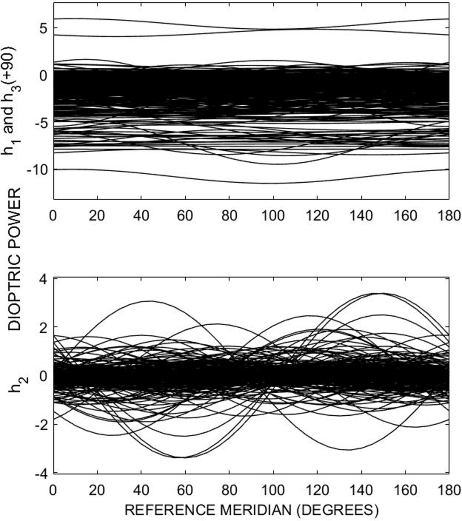
It is possible to build any power, including asymmetric powers, using just cylinder powers1 and therefore it is tempting to think of cylinder powers as the most basic power providing a rationale for basis γ . Coordinate vector h is a more direct measure of surface shape and thus is useful for analysis of both power and curvature of single refracting surfaces such as the anterior cornea.1 However, symmetric dioptric power F and basis β ‘better reflects the inherent symmetry of SDPS’1 and is better aligned to understanding the nature of characteristic structures2 that one can define in SDPS. Coordinate vector f and basis β is used to study refractive behaviour as it easily allows for analysis of meridional variation in power (see figure 2).

Meridional profiles of dioptric power for the Near Eye Tool for Refractive Assessment refractive states for the right eyes of 279 participants, aged 9–63 years. Curvital powers are shown in the upper plot with torsional powers in the lower plot. This is the same sample as in figure 1. (Data courtesy of NH—see reference number 64).
Advantages of stereo-pairs
Why then is a stereo-pair an advantage over other methods of graphical representation of symmetric dioptric power or refractive behaviour? Symmetric dioptric power is 3D and thus is only fully represented graphically on a 3D plot. Stereo-pairs allow for the 3D plot to be viewed stereoscopically such that relationships between the three building blocks (or component parts) of power are easily seen; much detail is lost when viewing a 3D plot two-dimensionally (eg, looking at only one half of the stereo-pair in figure 1A). In addition, to plot only two axes and ignore one, for example, to view the antiscalar (antistigmatic) plane by viewing along the M-axis (such as in figure 1C) one loses the relationship of astigmatism to the scalar component.
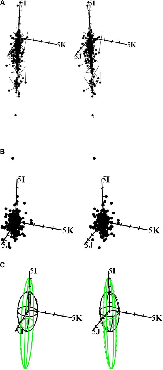
The distributional plot (of data) alone without SCPD is the most fundamental, simple and holistic method for representation of the distributions of such data and is not really affected by data normality or sample size; data can be normal or non-normal and still fully understood. Individual measurements (powers) can be seen in proper position relative to one another in 3D SDPS and magnitude, direction of variation and departures from normality and outliers are easily assessed; this is not always the case with other methods of graphical representation of power. Many methods in SDPS can be used to study pretreatment and post-treatment results or anisometropia such as the comets (figure 3A) and excesses or differences (figure 3B) as illustrated later. In summary, power matrices F are complete and holistic while power vectors may provide only partial solutions to clinical and research questions.

Stereo-pairs for 279 right and left eyes: (A) Comets OD to OS (non-reflected); dots at the start of comets represent OD while ends of comets represent OS, (B) excesses or differences for OD and OS (non- reflected) with a 95% confidence ellipsoid for the mean (CEM) (near origin) that cannot be seen as the dots are obscuring the very small CEM, (C) Distribution (95%) and confidence (95%) ellipsoids for the excesses (points not shown) of OD and OS. Black is used for ellipsoids before reflection and green for ellipsoids after reflection of the cylinder axes for OS. There are therefore four ellipsoids, that is, both with and without reflection of cylinder axes for OS. (Data64 courtesy of NH). OD is oculus dexter (right eye) and OS is oculus sinister (left eye).
A brief review of clinical applications using effective analysis of dioptric power
Over the last three decades general analyses for dioptric power globally have improved and it is now rare that journals will readily accept papers that do not use either power vectors2–6 10–22 24 26–39 (such as those of Harris2 or Thibos et al 24 or others such as Alpins32 33 or power matrices.1 10–22 25 27–31 41–74 This section will very briefly summarise applications where such methods are used in ophthalmology and optometry. The search strategy applied is explained in greater detail below.
Ophthalmic surgery and disease
There have been profound advances in ophthalmology and ophthalmic surgery in the late 20th and 21st centuries and particularly involving refractive surgeries and intraocular implants41 for conditions such as cataract42–46 that has rapidly increased in prevalence80 as the world’s population has also increased. Similarly, refractive surgery has become important for treatment of myopia, hyperopia, astigmatism and presbyopia. Many ophthalmic diseases and particularly astigmatism81–84 and corneal diseases such as keratoconus,85 86 have major implications for refractive behaviour and precision and predictability of surgery is important in improving surgical outcomes and patient satisfaction.
Thus, effective analysis of corneal and lenticular power and power of the eye itself has become paramount. Corneal surgeries,85–95 including for pterygia88 and implants89–92 and their effects, with or without other forms of ophthalmic surgery such as LASIK81 83 or SMILE,95 have been studied using power vectors. The same applies to surgical treatment with IOL.96–109 Given the diversity of human response and healing, satisfactory statistical methods are necessary to make correct decisions and advance surgical and other methods of treatment (eg, genetic or drug-related) for such ophthalmic conditions and diseases. Surgical treatments for glaucoma110 or other retinal anomalies such as retinal detachment, strabismus,111 112 or eyelid disorders113 also affect refractive behaviour with changes in astigmatism specifically.
Effective analyses of dioptric power, although mostly with power vectors or Alpins vector analysis32–35 104 rather than power matrices, have been applied to diverse topics including keratoconus and its surgical treatment via collagen cross-linking105 or methods such as LASIK or astigmatic keratotomy (AK), sometimes involving corneal grafts or IOL. Power vectors have also been used for analysis of postsurgical astigmatism and, for example, Mol and Van Dooren recently85 investigated 17 eyes of 16 patients (mean age and SD; 60±11 years) with toric IOL implantation after phacoemulsification. These eyes all had pre-existing astigmatism of relatively large magnitude (mean cylinder of 6.7 D) relating to either keratoconus or surgery for pterygia or after keratoplasty. Twelve months after toric IOLs were implanted mean refractive cylinder power was 1.5 D as determined with vector analysis while mean scalar (spherical) power or nearest equivalent sphere (M=F I) and SD were 0.25±1.53 D. So, surgery and toric IOL markedly reduced pre-existing cylinder (F c) and spherical power (F s) in most eyes concerned but there were outliers or eyes where the treatment was less successful and postsurgical or residual astigmatism was still a concern. Among other factors such as visual acuity, they85 used astigmatic vectors to represent cylinder power before and after toric IOL implantation in the Jacksonian or antiscalar plane (the J 0-J 45 or F J-F K plane) but without confidence ellipses for the eyes concerned. A similar approach with power matrices would involve stereo-pairs, SCPD and comets from the presurgical to postsurgical refractive state; and examples of such plots are included herein; however, F I (=M), or scalar coefficients of power are not excluded from these plots as in Mol and Van Dooren.85
Ophthalmic biometry and physiology
Power vectors and sometimes power matrices have been used to explore ophthalmic biometry such as axial length in relation to refractive state and also to study and quantify corneal power or curvature of both the anterior and posterior surfaces of the cornea and, for example, Liu et al
114 used power vectors and bivariate confidence regions to investigate age and astigmatism as well as any association between internal astigmatism and lenticular opacification and they found only a weak but significant association ( ) corrected for age, sex and type of cataract. They plotted distributions of J
0 and J
45 with confidence ellipses for the right and left eyes of their sample. (Their ellipses are 2-dimensional as against the three-dimensional SCPD as in figure 1A.) The antiscalar plane (that contains the two axes above) can be viewed directly by rotating stereo-pairs (see figure 1C) to look along the scalar axis. The advantage of the latter is that the scalar or spherical powers are directly included (in figure 1C) rather than excluded such as in Lui et al.114
) corrected for age, sex and type of cataract. They plotted distributions of J
0 and J
45 with confidence ellipses for the right and left eyes of their sample. (Their ellipses are 2-dimensional as against the three-dimensional SCPD as in figure 1A.) The antiscalar plane (that contains the two axes above) can be viewed directly by rotating stereo-pairs (see figure 1C) to look along the scalar axis. The advantage of the latter is that the scalar or spherical powers are directly included (in figure 1C) rather than excluded such as in Lui et al.114
Uncompensated refractive state (URE) is a worldwide problem115 116 producing unnecessary visual impairment (VI) irrespective of age117–119 and power vectors and matrices and other methods herein are necessary in understanding and developing effective and optimal means to address URE. For example, a recent paper120 by Rampat et al uses artificial intelligence or machine learning and wavefront aberrometry to predict subjective refractions (SR) for 3729 eyes. Power vectors are used in the initial stages of their analysis. One of their intentions was to develop methods for optimisation and objectively deciding on suitable spectacle prescriptions for patients based purely on wavefront aberrometry, and hence reduce the need for time-consuming SR that also requires a higher level of skill than, say, simply using an aberrometer for measurement of SR. There are also, naturally, concerns as to reliability and precision of SR whatever the method applied.114 120–124 So, Rampat et al were interested in establishing a new gold standard for clinical measurement of refractive error from lower order aberrations.120 Given the very large amount of unnecessary VI globally115 116 simply relating to URE (≈153 million in 2004116 and an estimated 1 billion in 2020116 finding an alternative to SR could be helpful. Rampat et al compared their predictive models to raw data for SR and their results were displayed in the antiscalar plane with 95% confidence ellipses for the different methods and their prediction errors were of small magnitudes (≤0.5 D) for the antiscalar coefficients at least.120 Whether this would also be true for M (=F I) for non-cycloplegic predictive refractions is another issue. However, their study certainly illustrates very effectively the usefulness of proper dioptric power analysis and its potential for incorporation into machine learning models and artificial intelligence for automated measurement of refractive behaviour.
Precision,121 reliability, reproducibility and agreement122 123 for measures122–124 to understand refractive behaviour of the cornea125 or eye,126 whether subjective or objective and with127 or without cycloplegia are also of interest in addressing the global increase in myopia and URE with subsequent VI. Anisometropia38 44 73 and interocular symmetry67 128 of the eyes of individuals are part of these areas of investigation and these aspects will be briefly considered later.
Variation in refractive behaviour in relation to physiological factors such as pregnancy,129 ocular accommodation30 31 or ageing62 63 101 117–119 have been investigated to some extent with power vectors or matrices. Epidemiological studies of the relevant components of the eye in terms of refractive state (and meridional refraction130 have also improved our understanding of the nature and variation of the cornea, air-tear interface and even the retina itself. This is an area where further research with large samples remains necessary although there are studies21 22 28 56 58 62–64 66–70 73 81 82 96 97 117–120 where power vectors or matrices are used to investigate distributions of refractive behaviour but they remain relatively few in number. Often sampling is not random13 and thus clinical or other biases may be limiting factors for such studies.
Myopic astigmatism
We have isolated this topic from the previous sections due to the rapidly increasing global prevalence of myopia and the large impact, now and in the future, that myopia is likely to exert on the global public health system and individual quality of life also.131 Moderate to severe myopia are important for effects in relation to foveal integrity and retinal nerve fibre layer thickness as well as factors such as retinal detachment.131 Treatments for myopia (such as refractive surgery, low-dose atropine, gene therapy, lenses and others)132–136 need further study with power vectors and matrices but studies are available and more emerge each year.
Although the emphasis in studies of myopic astigmatism is towards understanding distributions of refractive behaviour and especially that relating to myopia, power vectors and matrices are also of interest when considering reliability, validity and precision of measurement instruments in relation to refractive behaviour. For example, Cervino et al 137 used power vectors to study instrument myopia in adults (mean age: 20.8±2.5 years) with three different wavefront analysers and a binocular open-view autorefractor (SRW-5000). Their sample was relatively small at 80 eyes (21 women and 19 men) and measurements were obtained without cycloplegia. They considered outliers and concluded there was slightly more myopia on average (0.3 D) with the wavefront aberrometers than with binocular open view autorefraction but, overall, they found good agreement across the different instruments and there were no significant inter-instrumental differences for the antistigmatic coefficients (F J =J 0 and F K=J 45). Detailed exploration of myopia is outside the scope of this paper but research over the last two decades has emphasised myopia and its consequences and management and power vectors and matrices are important in that regard.
Methods
Search strategy and study selection
A literature search for relevant papers was done mainly with MEDLINE via the Web of Science. The following general search strategy was used: (power vectors OR power matrices) AND (refractive state OR refractive error). This yielded 185 papers over the timespan (1970–2021) concerned. Further searches for more specific papers to the topics of eye surgery, eye disease or ocular disease and transformations of dioptric power and outliers were also performed. Titles and abstracts were screened for relevance and full-text manuscripts were obtained as required. We only included papers with appropriate methods for analysis of dioptric power and refractive state, namely either power vectors or power matrices. Papers where the methods for analysis of dioptric power and refractive state were unclear or other methods used, such as analysis of spherical equivalents only, were excluded.
Statistical analysis of dioptric power
One of the first considerations in statistical analysis must be an exploration of the nature of the sample under investigation. For example, is the data normally distributed and are there possible outliers present? Various methods (see figures 1, 2 and 4) are available for this initial assessment of refractive data. Thereafter transformations of data and/or removal of outliers might be considered before proceeding with the analysis. Then a decision is made as to whether mainly parametric or non-parametric methods should be applied. Hypotheses and their evaluation for refractive behaviour12 13 15 also become an important element in the analysis. Presently, although some methods (see later) are available, there remain uncertainties within the field of statistical analysis of dioptric power and consequently of refractive behaviour.
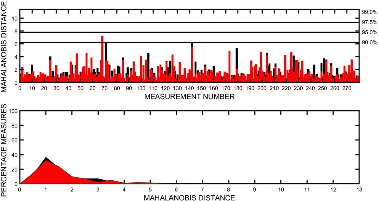
Mahalanobis distances (MD) for the same samples as in previous figures are provided for OD (black) and OS (red) bars in the upper rectangular plot with confidence levels as indicated at the top right of plot. The lower plot indicates that, irrespective of laterality (OD or OS), most eyes had MD <2. OD is oculus dexter (right eye) and OS is oculus sinister (left eye).
In terms of refractive behaviour and transformations of data that are not normally distributed, usually one begins with the weakest transformation (the square root transformation) and then proceeds towards the strongest transformation (the inverse or reciprocal transformation).21 22 Transformations are, however, not necessarily always advisable, and thus one needs to understand the effects of such transformations. Different approaches can be applied but for simplicity only Mardia’s23 multivariate skewness and kurtosis will be used here.
Results
Fundamental analysis of refractive behaviour
The specific aim below is to relate the analysis of dioptric power using both power vectors and matrices27 and to emphasise a few critical issues also such as departure from normality,21 22 138–141 outliers21 22 and transformations21 22 of data. These important issues are often ignored in analyses.64 The analysis is brief, but the key aspects, methodology and their relevance should become readily apparent. Included in the analysis are plots illustrating fundamental elements for analysis of refractive behaviour and figure 1A,B indicate the refractive states of 279 right eyes as measured using the Near Eye Tool for Refractive Assessment (NETRA) which is a cell-phone based, mixed subjective and objective method for determination of refractive behaviour. The methodology is described elsewhere,64 but a few points will be included here to assist readers with the necessary context. The sample involves participants in the age range, 9 to 63 years (with mean age and SD of 22.6 ± 8.9 years), predominantly of African descent (49.1%) and female (66.7%) and measurements were obtained without cycloplegia.
With exclusion of the SCPD,13 17 18 the stereo-pair scatter plot (that is, the data points only) of figure 1A (using h-vectors) and 1b (using power matrices, F i where i=1:279 here) are the most fundamental graphical representation of dioptric power and assumptions of normality are not an issue with such representations (although SCPD assume data normality and are influenced by outliers). In figure 1C the axes are rotated to view along the scalar (spherical) axis (which advances towards the observer using an exo-posture during fusion). Effectively this orientation allows one to view the antiscalar plane (containing the two antiscalar axes with labels 5J and 5K here). This plane contains all possible powers that are antiscalar or Jacksonian (ie, JCC). Over the previous decade or two, many studies of refractive state have emphasised this plane using power vector t with axes J 0 and J 45 and equating this plane with astigmatism. This method, however, ignores the fundamental multivariate nature of refractive state and while this approach is not incorrect, astigmatism cannot be simply equated with antiscalarism (or antistigmatism) and one also cannot ignore the scalar components of power as is sometimes the case. Powers are either scalar (spherical) or astigmatic (anything that is not scalar including antiscalar powers) and they are respectively found on the scalar axis (with label 5I, for example, in figure 1B or are located away from the scalar axis and are astigmatic. Antiscalar (or antistigmatic) powers are simply JCC found within a single plane within the infinite 3-space of all symmetric powers concerned (ie, a subspace of four-dimensional dioptric power space).1
In table 1, means and variances and covariances for the right (figure 1) and left eyes for the NETRA are provided. The centre (or centroid) of each 95% SCPD (or distribution ellipsoid) in figure 1 is the sample mean for OD.
If one instead uses power vectors (f or t) then one or more separate plots are required for coefficients, M, J 0 and J 45, and this is commonly used in papers involving refractive state or coefficients are combined in a single plot, however such plots become quite cluttered as a result. Alternatively, we can use two pseudo-3D plots as in figure 1D to create a stereo-pair. Such plots can be rotated to view the antiscalar plane. So, stereo-pairs as in figure 1 provide a single stereoscopic plot once fusion occurs and this greatly simplifies analysis and interpretation of the data. The axes in such figures represent the scalar and antiscalar powers and readers can think of the three axes as M I, J 0 J and J 45 K or as we prefer F I I, F J J and F K K where M=F I, J 0=F J and J 45=F K. The crucial difference here is not what symbols are used to label the axes but rather that figure 1B, for example, is a representation of a small part of an infinite Euclidean 3-space where points each represent a unique 2×2 power matrix, F i (see equation 20). The axis labelled F I I (=M I) is the scalar axis and here we can see that the NETRA refractive states cluster near this axis, mostly ranging from I (the first tick on the positive part of the vertical axis) to approximately −10I D (the continuation of the axis in the negative power direction). That is, this sample contains refractive states that are mostly myopic with small amounts of astigmatism. The greater the cylinder (in clinical terms), the further away from the scalar axis is the point for that power matrix.
It may be difficult for some people to fuse stereo-pairs and so the same sample is shown in figure 2 using meridional profiles of dioptric power. They are less satisfactory as each power is represented by three profiles (two are shown on one rectangular plot with displacement of 90°) rather than a single point in the stereo-pairs in the previous figure. Nonetheless, they are often helpful to identify outliers and departures from normality and study the nature and magnitude of sample variation and they are in many ways supplemental and complimentary to the stereo-pairs. Both methods are complete representations of the distribution concerned.
Outliers and Mahalanobis distances
In figure 1B, there are three points (two near the label 5I and one far beyond −5I) and these are respectively three eyes, in clinical terms, with refractive states near 5 D of hyperopia and −10 D of myopia. Should we regard these eyes as outliers and perhaps remove them from the sample? Outliers and how to manage them in samples should always be considered prior to data collection and at the start of the analytical process. So, what should we do about possible outliers in samples such as in figure 1A,B and also figure 2 where atypical profiles can be identified? One approach is to use Mahalanobis distances (as in figure 4) where only 2–4 measurements (bars) reach the 90% level of confidence; so, outliers are uncommon in the sample concerned. Mahalanobis distances ( ) are the distances between points in a distribution and their mean. The greater the distance the more probable a point is to be an outlier and the greater are the numbers of SD of that point away from the respective mean. Thus, Mahalanobis distances are useful in multivariate outlier detection. In terms of coordinate vector f:
 (35)
(35)
The subscript index i=1 to N is used for the sample measurements,  and S are the sample mean and variance–covariance matrix, respectively. (Coordinate vector h could be used in equation 35 instead of vector f.)
Where the population distribution is not known, another method would be to use the Chebyshev inequality141 to estimate the probability that specific measurements differ from their mean by more than a specified number of SD. Stellato et al 141 also derive a multivariate form of the Chebyshev inequality that uses the Euclidean norm or Mahalanobis distance for outlier detection141 but, for simplicity here, the univariate Chebyshev inequality is141:
 (36)
(36)
and equation 36 provides the probability (
P
) that a scalar and random variable (
ξ
) with distribution
P
differs from its mean (µ) by more than a specified number (λ) of SDs (σ) with the condition  , that is, the number of SD is real and positive, and that the probability is less than or equal to the minimum as specified in equation 36. There are some difficulties with this inequality as we are usually not sure of the true values of the population means and variances, and thus they need to be estimated via sampling and this process might not always provide satisfactory estimates. Also, the inequality is sensitive to sample size and the number of samples concerned in estimation of the means and SD. (These limitations would, however, apply also to that of figure 4 where Mahalanobis distances (equation 35) are provided for the sample concerned.
Data normality and transformations to normality
The nature of distributions and possible transformations of data for dioptric power and refractive behaviour are relatively unexplored in the literature although some work21 22 31 62 in this direction can be found. Normality of samples is important with statistical methodology such as SCPD17 18 and univariate or multivariate hypothesis tests.12 13 15 This paper will introduce the topic but will not include a detailed exploration. There are several methods to transform univariate or multivariate data and one of the most common is a square root transformation. However, if this is attempted for dioptric power data then we find that negative quantities (for myopes) produce results that need to be analysed in a complex space. Plotting results and analysing such transformed data then becomes interesting as one needs to use power components (F I, F J and F K or respectively, M, J 0 and J 45) in the complex plane and stereo-pairs of power matrices that involve complex numbers, which to the best of our knowledge has not been used previously with analyses of dioptric power. If, instead, to avoid such issues and leave them for the future, we attempt a simple log transformation we encounter the same problem with imaginary numbers. One answer is to use shift transformations21 22 to convert all negative values in the data to positive values. Where a value is added to the data different power transformations for different coefficients of power (F I, F J and F K) can be used and, of course, the same applies with vector t. Alternatively, we might proceed with an inverse transformation where negative powers would not be a problem. Once such transformations have been applied and normality has been assessed with normality plots21 22 or other methods23 then a reverse transformation is necessary to move the data back towards its initial representation in SDPS.21 22 For a more comprehensive consideration of transformations of dioptric power, references 21 and 22 are relevant.
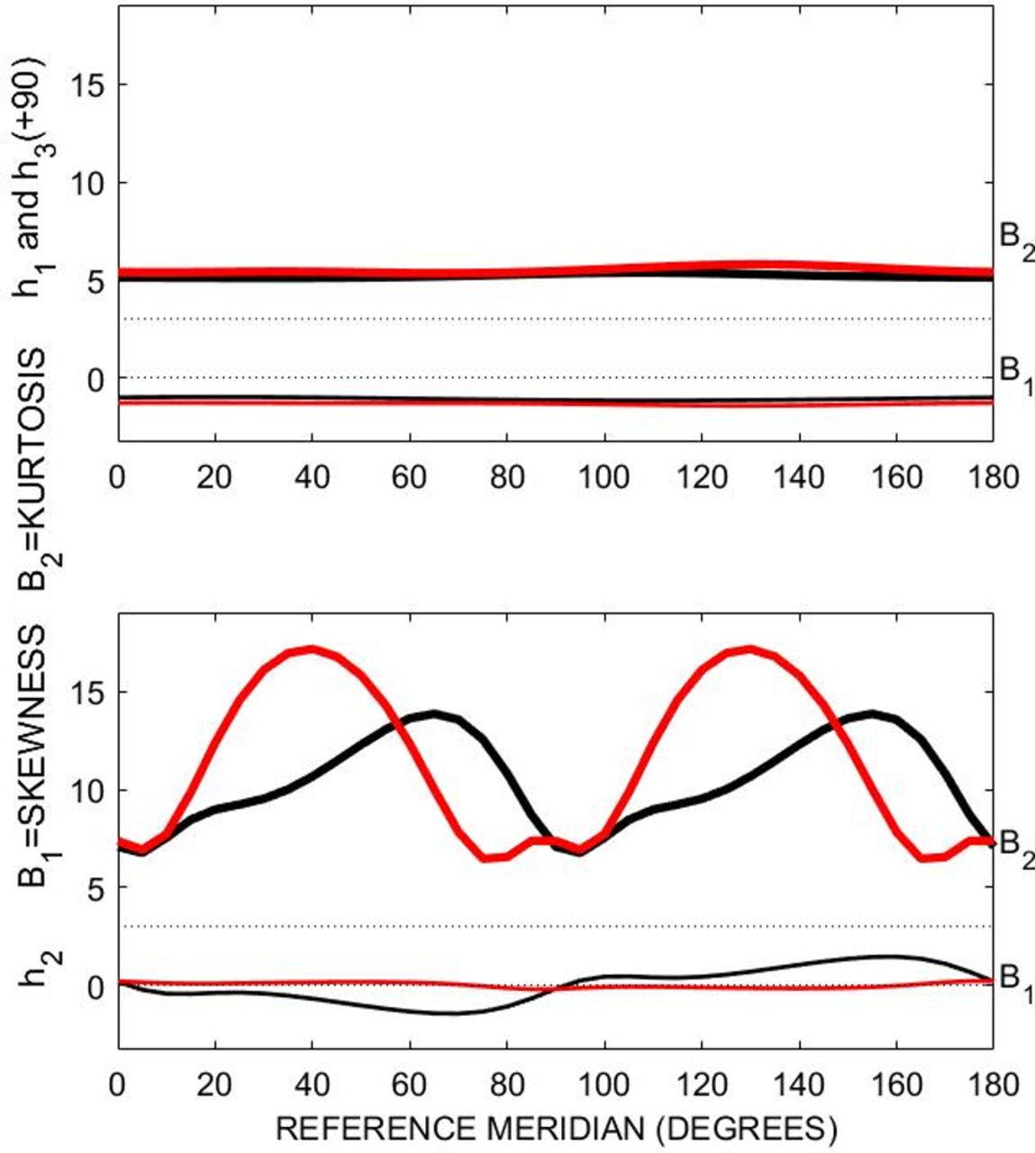
An alternate approach is to calculate univariate or Mardia’s23 multivariate moments of skewness and kurtosis and use meridional profiles for skewness and kurtosis such as in figure 5 where the same data as for the previous figures are used. This approach is also useful to evaluate the effects of removal of possible outliers. In figure 5 almost uniform leptokurtosis (B
2>3) and mild negative skewing (B
1<0) is noted for the curvital coefficients (h
1 and h
3) of power but both mild positive (B
1>0) and negative skewing (B
1<0) is seen for the torsional coefficients (h
2) of power. Non-uniform meridional variation in leptokurtosis is obvious for h
2. Thus, the SCPD in figure 1 and the variances and covariances in table 1 need to be treated with caution as they assume data normality which is not the case here. We could do transformations and/or remove possible outliers and then examine multivariate moments of skewness and kurtosis and perhaps replot figure 5 that might demonstrate greater normality (using univariate moments of skewness and kurtosis) but that and other procedures using normality and  plots21 22 are outside the scope for this paper. Nonetheless, effective analysis of dioptric power and refractive behaviour cannot be done without consideration of outliers and data normality.

Meridional profiles of skewness ( ) and kurtosis (
 ) for 279 right (in black) and left (in red) eyes of the same participants as for figure 1. The dotted lines represent the expected values for skewness (=0) and kurtosis (=3) for univariate normal distributions. Although vector
h
is used here,
) for 279 right (in black) and left (in red) eyes of the same participants as for figure 1. The dotted lines represent the expected values for skewness (=0) and kurtosis (=3) for univariate normal distributions. Although vector
h
is used here,
 ,
,
 and
and  . Thus, the top plot indicates these statistics for the curvital coefficients of power (h
1 and
. Thus, the top plot indicates these statistics for the curvital coefficients of power (h
1 and  ) while the bottom plot is for the torsional coefficients (
 ) of power and they relate to the corresponding symmetric power matrices
  where i =1:279 here. (Data64 courtesy of NH).
Variances and covariances for refractive behaviour
For any sample of dioptric powers, measures of central tendency11 13 and dispersion or variation10–13 are important and, for example, in table 1 variance–covariance matrices10–12 are given. They are, however, incomplete in that they only provide an understanding of variation in relation to the three axes as illustrated, for example, in figure 1B. With dioptric power, the issues around variation are more complicated with an infinity of possible directions for variation in the Euclidean 3-space (here SDPS). Consequently, meridional14 19 29–31 or polar profiles30 31 (such as in figure 6) for variances and covariances are necessary and they inform us about variances in all meridians for the sample concerned. In figure 6, curvital variances are similar or uniform (≈4.5 D2 or equivalent to SD of  for all meridians but slightly less so for the right eyes (the outer black profile in figure 6). Torsional variances are almost zero (see the two profiles near the polar origin and although they are slightly variable across meridians the profiles are not significantly different and we would need to reduce the radial scale of 6 D2 to better observe these profiles.) The covariances (that indicate linear covariation between pairs of coefficients for power) are not included in figure 6 but see references 30 and 31 by van Gool and Harris.

Polar profiles of curvital (outer profiles for f
11 and f
22 (+90)) and torsional (f2
1 = f
12) variances (inner profiles near polar origin) for the right (in black) and left (in red) eyes of 279 participants, aged 9–63 years are provided. Variances for f
11 and f
22 are shown on the same profiles (red or black) but with a separation of 90° within profiles. There are four profiles but the two torsional profiles overlap and one cannot easily distinguish any differences between the black and red torsional profiles. The outer profiles are almost semicircles of constant radius and curvital variances are similar for the right and left eyes with respect to change across meridians. These profiles are used to understand the variation of power along meridians as well as to obtain quantities of interest such as meridians of maximum and minimum variance. The azimuthal scale is 0:180° and the radial scale is (0:1.5:6  ) and small numbers at 3 and 6
  on the vertical meridian can be seen (data 64 courtesy of NH).
Anisometropia
Differences in refractive behaviour across eyes and between individuals38 39 44 67 73 114 128 are of importance in analyses of dioptric power and the following briefly considers some methods towards qualitatively and quantitatively analysing anisometropia.44 67 73 Anisometropia and aniso-astigmatism are often a consequence of conditions such as keratoconus69 70 85 86 105 123 but can also be an important consideration in refractive42–44 74 87 125 or other surgeries42–44 87–113 sometimes involving IOL36 41–43 45 46 85 99–104 or other implants.89–92 105 Reliability and reproducibility of measures of refractive behaviour are integral to understanding anisometropia.40 57–64 66 109 120–123 Ocular accommodation,21 22 28 30 31 54–58 62–68 70 73 127 outliers, departures from data normality, laterality and mirror symmetry67 95 and reflection of cylinder axes2 11–13 15 17 18 28 67 73 74 must be considered in effective analyses of anisometropia.
Without going into too much detail here, in figure 3A comets are used to join the refractive states of the right and left eyes of each of the 279 participants. The shorter a comet the greater the agreement or similarity (isometropia) between the refractive states for the two eyes of a participant and if there was perfect isometropia for a participant a point would be seen instead of a comet. Although not included here, the Euclidean lengths of the comets can be used to determine measures such as mean length and SD and these can be applied to quantification of anisometropia. In figure 3A the cylinder axes for the left eyes are non-reflected. With mirror symmetry and anisometropia, reflection of axes of left eyes (180-A where A is the cylinder axis could be applied to each participant) when comparing the right and left eyes and that could affect directions and lengths of comets such as in the figure 3A. In figure 3B, matrices were used to determine excesses (or differences) between eyes of each participant. The origin is the null matrix, O D, that is, no difference or an excess of zero. If isometropia is present for a participant a point at the origin would be found. (Note the large excess above the label (5I) for the scalar axis; this point represents a participant where anisometropia was profound.) Although not obvious in figure 3A,B a 95% confidence ellipsoid for the mean18 (CEM) is also included and its volume and centroid (the mean excess or difference) are important regarding classification of anisometropia. This CEM is more obvious in figure 3C where, for clarity, the points (excesses) are not included and the CEM is the very tiny black ellipsoid just below the origin of the three axes.
Figure 3C includes two larger distribution ellipsoids (or SCPD) for the excesses, before (in black) and after reflection (in green) of cylinder axes for OS while the two smaller ellipsoids are 95% CEM for the same data, again before (in black) and after reflection (the very small green ellipsoid with an almost vertical linear structure that is located about 1.5 D below the origin and that spans the central cross section - see the small green ellipse - of the larger green ellipsoid.) Although not within the scope of this review, quantification of the excesses can be applied to further understand anisometropia for the data concerned.
Discussion and conclusions
Although hypothesis tests for dioptric power and refractive behaviour were not included here for the explanatory analysis, means and variance–covariance matrices10 11 can be compared using univariate11 13 15 or multivariate hypothesis tests11–13 15 138–141 and statistical conclusions for refractive behaviour can be made. For example, whether there is a statistically significant difference in means between the right and left eyes or whether the variance–covariance matrices (for example, as in table 1) are equal or not. Various assumptions such as data normality and equality of population variance–covariances are important.10–13 15 17 18 21–23 141
This review has highlighted some potential weaknesses in the literature for analysis of dioptric power and refractive state and has used data to illustrate important concerns that should be considered in any analysis of dioptric power. Often analyses place emphasis on astigmatism without due consideration for scalar powers or the holistic and multivariate nature of refractive state and its variation or behaviour. Similarly, sometimes scalar powers are emphasised without due attention to astigmatism. In general, the concepts of antistigmatism are confused with astigmatism and analysis is generally confined to the antistigmatic (antiscalar or Jacksonian) plane that is occasionally called the astigmatic plane, a phrase that is somewhat confusing. In this area of study, most papers in ophthalmology and optometry do not use stereo-pairs and this complicates interpretation and understanding of dioptric power and refractive behaviour. SCPD13 17 18 or other measures of uncertainty such as error cells around powers71 72 are often absent from analyses. While bivariate CIs are sometimes used24 82 114 130 they are not always applied with due regard to possible outliers and their significance or to the nature of distributions and possible departure from normality.21–23 Consideration of outliers21 22 28 30 31 56–70 73 74 138 and the use of trivariate CIs13 17 18 20–22 24 26 28 30 31 38 39 55–70 73 74 82 that are fundamental to understanding symmetric dioptric power and refractive behaviour are not used as often as necessary. Hypothesis tests are sometimes included in papers but occasionally without due regard to assumptions underlying such statistical tests. This paper has attempted to illustrate some of the necessary procedures and concerns that should be considered in effective analyses of dioptric power and refractive behaviour. Many of the concerns about outliers21 22 and their proper identification and management in analyses remain for future investigation and the same applies to understanding distributions of refractive state and their normality or otherwise and where necessary possible transformations21 22 of data towards greater normality. Nonetheless, much of the methodology as applied here and elsewhere for the basic analysis of dioptric power and refractive behaviour has advanced significantly from that in the past. Recent papers142 143 use power vectors and second derivatives of dioptric power curves143 to study variation of power and thus imaging over the retina as induced by fractal contact lenses (basically a multizone bifocal design) and these lenses and similar spectacle144 lenses are likely to be important in reducing the progression of myopia in younger eyes that is an increasing problem possibly relating to insufficient time spent outdoors145 and too much activity with tablets, mobile phones and other online media often with small screens, sometimes held at close distances for lengthy periods. New methods for objective and/or subjective ophthalmic refraction120 124 146–148 with some based on remote measurement of refraction via the internet148 and their analysis and understanding also use vectors124 147–153 or matrices64 68–70 for dioptric power and astigmatism.149 150 Given the need to address the ever-increasing prevalence of myopia and its associations61–63 131 132 154 and potential risks to ocular and retinal health relating indirectly to changes in axial length147 over time and the consequent economic and social cost implications of myopic-related disorders such as maculopathy and retinal detachment, methodology to better understand and analyse data of this type and its management91 131–136 143–145 155 are important in preventing unnecessary vision impairment and human affliction and suffering.
Data availability statement
Data are available on reasonable request.
Ethics statements
Patient consent for publication
Ethics approval
This study involves human participants and was approved by HDC01-57-2016 and REC01-184-2016, Faculty Higher Degrees and Research Ethics Committees, Faculty of Health Sciences, University of Johannesburg, South Africa. Participants gave informed consent to participate in the study before taking part.
Acknowledgments
We thank Professor WF Harris for reading and commenting on the paper.
References
Footnotes
Contributors All authors contributed to the concept, preparation and writing of this review. NH contributed data from her DPhil study that was used in analysis herein.
Funding The authors have not declared a specific grant for this research from any funding agency in the public, commercial or not-for-profit sectors.
Competing interests AR, TE and NH were authors on some of the references as included in this review.
Provenance and peer review Commissioned; externally peer reviewed.
Linked Articles
- Vision Science
- Editorial
- Review